Locating position for certain size of complexes by PDB/restart file
By PDB file
locate_pos_no_restart(FileNamePdb, NumDict, FileNameInp, BufferRatio=0.01, OpName=”output_file”)
Description: This function allows users to locate specific complexes of a certain size from a PDB file after simulation. The result is output as a new file named output_file.pdb containing only the desired complex.
Parameters:
FileNamePdb (str): The path to the PDB file, typically the last frame of the simulation.
NumDict (dict): A dictionary that holds the requested number of protein types in a complex.
FileNameInp (str): The path to the .inp file, which usually stores the reaction information.
BufferRatio (float, optional, default=0.01): The buffer ratio used to determine whether two reaction interfaces can be considered bonded.
OpName (str, optional, default=”output_file”): The name of the output file.
Returns:
.pdb file: A PDB file containing only the selected complexes.
Example:
import ionerdss as ion
ion.locate_pos_no_restart(FileNamePdb = "nerdss_output.pdb", NumDict={"dod":9}, FileNameInp="parm.inp", OpName = “output”)
>>> Output_file.pdb that includes only proteins in complexes of the selected size
...
ATOM     19  COM dod    3      301.720 116.470 306.361     0     0CL
ATOM     20  lg1 dod    3      315.636 126.000 315.231     0     0CL
ATOM     21  lg2 dod    3      312.386 125.024 293.086     0     0CL
....
By restart.dat file
locate_pos_restart(FileNamePdb, NumDict, FileNameRestart, OpName=”output_file”)
Description: This function enables users to locate specific complexes of a certain size from a PDB file along with a restart.dat file after simulation. The result is output as a new file named output_file.pdb containing only the desired complex.
Important Note: The advantage of reading the restart.dat file is that it directly stores the binding information of each complex in the system, allowing the function to run faster. However, this function is not universal; if the write logic of the restart.dat file changes, the function will no longer work.
Parameters:
FileNamePdb (str): The path to the PDB file, typically the last frame of the simulation.
NumDict (dict): A dictionary that holds the requested number of protein types in a complex.
FileNameRestart (str): The path to the restart.dat file.
OpName (str, optional, default=”output_file”): The name of the output file.
Returns:
.pdb file: A PDB file containing only the selected complexes.
Example:
import ionerdss as ion
ion.locate_pos_restart(FileNamePdb="nerdss_output.pdb", NumDict={"dod": 9}, FileNameRestart="restart.dat", OpName="output")
>>> Output_file.pdb that includes only proteins in complexes of the selected size
...
ATOM     19  COM dod    3      301.720 116.470 306.361     0     0CL
ATOM     20  lg1 dod    3      315.636 126.000 315.231     0     0CL
ATOM     21  lg2 dod    3      312.386 125.024 293.086     0     0CL
ATOM     22  lg3 dod    3      294.395 112.226 289.287     0     0CL
....
Analyzing .xyz files
.xyz files hold the location of every protein at specific times. (Does not necessarily include every timestamp, more to compare a couple of timestamps).
CSV – creates spreadsheet of protein locations
xyz_to_csv(FileName, LitNum, OpName=”output_file”)
Description: This function converts the output .xyz file from a NERDSS simulation into a .csv file for a specific or entire time frame. The generated .csv file will contain 5 columns: iteration number, species name, and x, y, z coordinates.
Parameters:
FileName (str): The path to the .xyz file, typically named trajectory.xyz.
LitNum (int, optional, default=-1): The iteration number to examine. If set to -1, the function will extract data for all iterations.
OpName (str, optional, default=”output_file”): The name of the output file.
Returns:
.csv file: A CSV file containing the specified trajectory data.
Example:
import ionerdss as ion
ion.xyz_to_csv(FileName="trajectory.xyz", LitNum=-1)
>>> output_file.csv containing the trajectory data
DATAFRAME – creates dataframe of protein locations
xyz_to_df(FileName, LitNum=-1, SaveCsv=True):
Description: This function converts the output .xyz file from a NERDSS simulation into a pandas.DataFrame for a specific or entire time frame. The generated DataFrame will contain 5 columns: iteration number, species name, and x, y, z coordinates. Optionally, the DataFrame can be saved as a .csv file.
Parameters:
FileName (str): The path to the .xyz file, typically named trajectory.xyz.
LitNum (int, optional, default=-1): The iteration number to examine. If set to -1, the function will extract data for all iterations.
SaveCsv (bool, optional, default=True): Whether to save the DataFrame as a .csv file.
Returns:
pandas.DataFrame: A DataFrame containing the specified trajectory data.
Example:
import ionerdss as ion
traj_df = ion.xyz_to_df(FileName="trajectory.xyz", LitNum=-1, SaveCsv=False)
>>> traj_df
   iteration name           x           y           z
0          0   ap   87.420620 -270.109172 -203.661987
1          0   ap   88.081526 -271.052470 -205.297038
2          0   ap   86.759715 -269.165874 -202.026936
3          0   ap  -58.647113  277.528515 -353.236112
...
MATRIX - tracks the trajectory of specific protein(s)
traj_track(FileName, SiteNum, MolIndex, SaveVars=False)
Description: This function enables users to track the center of mass (COM) coordinates of one or more molecules over time. The return will be a 2D matrix with the size of the number of iterations times the number of desired molecules.
Parameters:
FileName (str): The path to the .xyz file, typically named trajectory.xyz.
SiteNum (int): The total number of COM and interfaces of a single molecule. For example, if a molecule possesses 1 COM and 5 interfaces, the SiteNum value should be 6.
MolIndex (list of int): The indices of the molecules to track. The numbers in the list should be no smaller than 1.
SaveVars (bool, optional, default=False): Whether to save the outputs in a file.
Returns:
Trajectory (list): A list containing the COM coordinates of the specified molecules at different time stamps.
Example:
import ionerdss as ion
trajectory = ion.traj_track(FileName="trajectory.xyz", SiteNum=3, MolIndex=[1, 4, 10])
>>> trajectory
[
    [[87.42062, -270.109172, -203.661987], [40.873538, 168.96348, -497.993163]],
    [[74.407358, 51.461467, -242.958456], [187.824563, 325.913499, -497.993163]],
    [[20.608487, 330.919045, -182.061499], [-27.367719, 330.945162, -497.993163]]
]
Analyzing .pdb files
LINE PLOT- Auto correlation function (acf) for complexes
acf_coord(PDBDirectory, mol_list, sim_num=1, time_step=1, show_fig=True, save_fig=False)
Description: Calculates the mean auto-correlation function (ACF) of protein complexes stored in a series of NERDSS-generated PDB files. If PDB files from multiple simulations are to be evaluated, they should be organized in the following directory structure before running the function:

Directory structure for ACF analysis.
Important Note: Given a series of .pdb files generated during NERDSS simulation, the function calculates the auto-correlation function (ACF) of the system. The ACF describes the correlation of a signal with a delayed copy of itself as a function of delay. In this context, it is the correlation of a complex’s position with its initial position as a function of time, calculated as the inner product between the initial position vector of a complex and its current position vector divided by the squared magnitude of its initial position vector:
Parameters:
PDBDirectory (str): The name of the directory where all PDB files are stored.
mol_list (list of str): The names of the molecules to be evaluated.
sim_num (int, optional, default=1): The number of repeated simulations to be evaluated.
time_step (int, optional, default=1): The time steps of the NERDSS simulation in microseconds.
show_fig (bool, optional, default=True): Whether to display the generated plots.
save_fig (bool, optional, default=False): Whether to save the generated plots.
Returns:
average_time_array (array): An array of iterations when the mean ACF over all repeated simulations is calculated.
average_acf_array (array): An array of the mean ACF calculated over all repeated simulations.
std_acf_array (array): An array of the standard deviation of the ACF calculated over all repeated simulations.
Example:
import ionerdss as ion
ion.acf_coord(PDBDirectory="testing_PDBs", mol_list=["A"], sim_num=2, time_step=0.1, show_fig=True, save_fig=False)
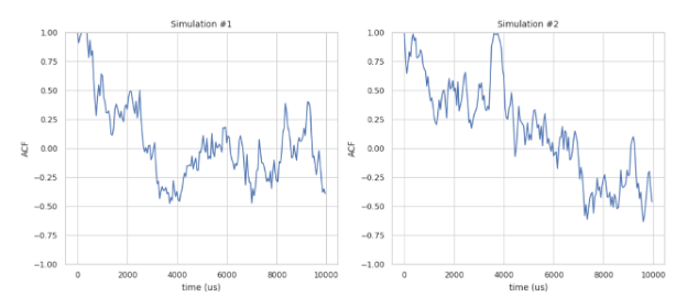
Separate ACF plots for each simulation.

Mean ACF plot over all simulations.